Day 1 AM: Introduction to R, RStuido and the data.frame
Using R and RStudio
R is a flexible language that is specialized for data analysis and
visualization. This workshop focuses on tabular data that can be
loaded into an R data.frame for exploratory analysis and
visualization. Other aspects of R, such as general purpose programming,
modeling for statistical inference and use of BioConductor for
specialized assay analysis are de-emphasized in this workshop.
Most people using R use it in the context of the RStudio graphical user interface (GUI) environment, and we introduce this environment to illustrate:
- The anatomy of RStudio
- The R console
- Writing, executing and “sourcing” R scripts
- Using R markdown and notebooks for literate programming
- Getting help
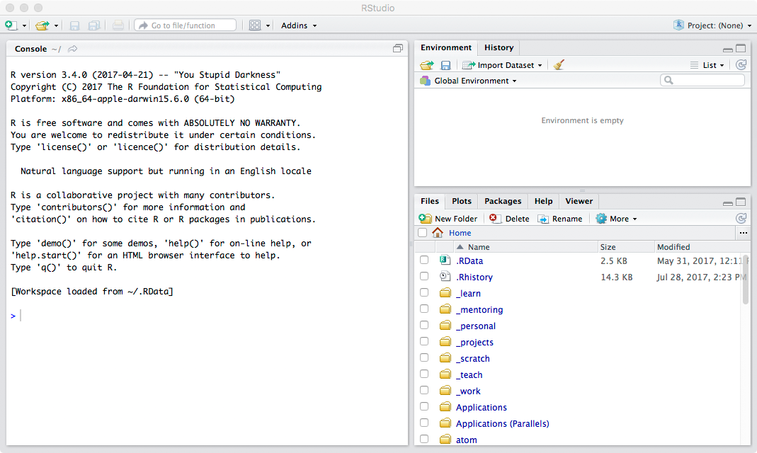
RStudio screenshot
Overview of the exploratory data analysis pipeline
The exploratory data analysis pipeline typically consists of the following steps:
- Converting messy data into tidy data
- Manipulating tidy data
- Visualizing tidy data
These actions are generally performed using the tidyverse
meta-package. We will cover the use of tidyverse and these stages in
reverse order in this workshop since the first two stages are quite dry
without setting up the correct motivation. First however, we cover some
essential concepts and show how data is loaded in the first place.
In [80]:
library(tidyverse)
Warning message:
“Installed Rcpp (0.12.12) different from Rcpp used to build dplyr (0.12.11).
Please reinstall dplyr to avoid random crashes or undefined behavior.”Loading tidyverse: ggplot2
Loading tidyverse: tibble
Loading tidyverse: tidyr
Loading tidyverse: readr
Loading tidyverse: purrr
Loading tidyverse: dplyr
Warning message:
“package ‘dplyr’ was built under R version 3.4.1”Conflicts with tidy packages ---------------------------------------------------
filter(): dplyr, stats
lag():    dplyr, stats
Types, collections and variable assignments
Strings
In [1]:
"This is a string"
In [2]:
substr("This is a string", 6, 10)
In [3]:
paste("gene", 1:10)
- 'gene 1'
- 'gene 2'
- 'gene 3'
- 'gene 4'
- 'gene 5'
- 'gene 6'
- 'gene 7'
- 'gene 8'
- 'gene 9'
- 'gene 10'
In [4]:
paste("Hello", "world", sep=", ")
Factors
In [10]:
sex <- as.factor(c("M", "F"))
In [11]:
sex
- M
- F
In [12]:
str(sex)
Factor w/ 2 levels "F","M": 2 1
Vectors
In [15]:
5:10
- 5
- 6
- 7
- 8
- 9
- 10
In [16]:
10:5
- 10
- 9
- 8
- 7
- 6
- 5
In [17]:
c(1,1,2,3,5,8)
- 1
- 1
- 2
- 3
- 5
- 8
In [18]:
seq(1, 10, by=3)
- 1
- 4
- 7
- 10
In [19]:
rep(1:4, 2)
- 1
- 2
- 3
- 4
- 1
- 2
- 3
- 4
In [20]:
rep(1:4, each=2)
- 1
- 1
- 2
- 2
- 3
- 3
- 4
- 4
In [21]:
rnorm(5, 100, 15)
- 102.594622335355
- 111.635958574435
- 103.443624575272
- 106.529771804924
- 85.6990987716058
In [22]:
sample(c("H", "T"), 5, replace = TRUE)
- 'T'
- 'H'
- 'H'
- 'T'
- 'H'
Matrices
In [23]:
matrix(1:12, nrow=4)
| 1 | 5 | 9 |
| 2 | 6 | 10 |
| 3 | 7 | 11 |
| 4 | 8 | 12 |
In [24]:
matrix(1:12, nrow=4, byrow=TRUE)
| 1 | 2 | 3 |
| 4 | 5 | 6 |
| 7 | 8 | 9 |
| 10 | 11 | 12 |
Lists
In [25]:
list(a=1, b=2)
- $a
- 1
- $b
- 2
In [26]:
list(a=5:10, b= 10:5)
- $a
- 5
- 6
- 7
- 8
- 9
- 10
- $b
- 10
- 9
- 8
- 7
- 6
- 5
Assignment
In [27]:
greet <- "hello"
In [28]:
greet
In [29]:
my.vec <- 5:10
In [30]:
my.vec
- 5
- 6
- 7
- 8
- 9
- 10
In [31]:
my.list <- list(a=5:10, b= 10:5)
In [32]:
my.list
- $a
- 5
- 6
- 7
- 8
- 9
- 10
- $b
- 10
- 9
- 8
- 7
- 6
- 5
In [33]:
my.matrix <- matrix(1:12, nrow=4, byrow=TRUE)
In [34]:
my.matrix
| 1 | 2 | 3 |
| 4 | 5 | 6 |
| 7 | 8 | 9 |
| 10 | 11 | 12 |
Indexing
Vectors
In [35]:
my.vec
- 5
- 6
- 7
- 8
- 9
- 10
In [36]:
my.vec[1]
In [37]:
my.vec[-1]
- 6
- 7
- 8
- 9
- 10
In [38]:
my.vec[-c(1,3)]
- 6
- 8
- 9
- 10
In [39]:
my.vec[2:4]
- 6
- 7
- 8
Lists
In [40]:
my.list
- $a
- 5
- 6
- 7
- 8
- 9
- 10
- $b
- 10
- 9
- 8
- 7
- 6
- 5
In [41]:
my.list$a
- 5
- 6
- 7
- 8
- 9
- 10
In [42]:
my.list[1]
- 5
- 6
- 7
- 8
- 9
- 10
In [43]:
my.list[[1]]
- 5
- 6
- 7
- 8
- 9
- 10
Matrices
In [44]:
my.matrix
| 1 | 2 | 3 |
| 4 | 5 | 6 |
| 7 | 8 | 9 |
| 10 | 11 | 12 |
In [45]:
my.matrix[2,3]
In [46]:
my.matrix[2,]
- 4
- 5
- 6
In [47]:
my.matrix[,3]
- 3
- 6
- 9
- 12
In [48]:
my.matrix[2:3, 2:3]
| 5 | 6 |
| 8 | 9 |
Getting data into a data.frame
Preloaded data.frame
R preloads several data sets that are often used as examples in R tutorials. To find out what these are, enter
library(help="datasets")
In [58]:
head(iris)
| Sepal.Length | Sepal.Width | Petal.Length | Petal.Width | Species |
|---|---|---|---|---|
| 5.1 | 3.5 | 1.4 | 0.2 | setosa |
| 4.9 | 3.0 | 1.4 | 0.2 | setosa |
| 4.7 | 3.2 | 1.3 | 0.2 | setosa |
| 4.6 | 3.1 | 1.5 | 0.2 | setosa |
| 5.0 | 3.6 | 1.4 | 0.2 | setosa |
| 5.4 | 3.9 | 1.7 | 0.4 | setosa |
In [59]:
head(faithful)
| eruptions | waiting |
|---|---|
| 3.600 | 79 |
| 1.800 | 54 |
| 3.333 | 74 |
| 2.283 | 62 |
| 4.533 | 85 |
| 2.883 | 55 |
Creating a data.frame from scratch
A data frame is just a collection of lists of the same length, where each list contains only one type of variable, is treated as a column.
In [56]:
n <- 8
my.df <- data.frame(pid=1:n,
                    sex=as.factor(sample(c("M", "F"), n, replace = T)),
                    iq=round(rnorm(n, 100, 15), 0))
In [57]:
my.df
| pid | sex | iq |
|---|---|---|
| 1 | M | 110 |
| 2 | F | 104 |
| 3 | F | 65 |
| 4 | M | 106 |
| 5 | F | 89 |
| 6 | F | 95 |
| 7 | M | 129 |
| 8 | M | 96 |
Loading from CSV or other tablular file
In [69]:
url <- "http://vincentarelbundock.github.io/Rdatasets/csv/datasets/Titanic.csv"
titanic <- read.csv(url)
In [70]:
head(titanic)
| X | Name | PClass | Age | Sex | Survived | SexCode |
|---|---|---|---|---|---|---|
| 1 | Allen, Miss Elisabeth Walton | 1st | 29.00 | female | 1 | 1 |
| 2 | Allison, Miss Helen Loraine | 1st | 2.00 | female | 0 | 1 |
| 3 | Allison, Mr Hudson Joshua Creighton | 1st | 30.00 | male | 0 | 0 |
| 4 | Allison, Mrs Hudson JC (Bessie Waldo Daniels) | 1st | 25.00 | female | 0 | 1 |
| 5 | Allison, Master Hudson Trevor | 1st | 0.92 | male | 1 | 0 |
| 6 | Anderson, Mr Harry | 1st | 47.00 | male | 1 | 0 |
We can aslo download and read in as local file
In [71]:
download.file(url = url, destfile="titanic.csv")
In [72]:
titanic.1 <- read.csv("titanic.csv")
In [73]:
head(titanic.1)
| X | Name | PClass | Age | Sex | Survived | SexCode |
|---|---|---|---|---|---|---|
| 1 | Allen, Miss Elisabeth Walton | 1st | 29.00 | female | 1 | 1 |
| 2 | Allison, Miss Helen Loraine | 1st | 2.00 | female | 0 | 1 |
| 3 | Allison, Mr Hudson Joshua Creighton | 1st | 30.00 | male | 0 | 0 |
| 4 | Allison, Mrs Hudson JC (Bessie Waldo Daniels) | 1st | 25.00 | female | 0 | 1 |
| 5 | Allison, Master Hudson Trevor | 1st | 0.92 | male | 1 | 0 |
| 6 | Anderson, Mr Harry | 1st | 47.00 | male | 1 | 0 |
Understanding the data.frame
Structure
In [75]:
str(titanic)
'data.frame':   1313 obs. of  7 variables:
 $ X       : int  1 2 3 4 5 6 7 8 9 10 ...
 $ Name    : Factor w/ 1310 levels "Abbing, Mr Anthony",..: 22 25 26 27 24 31 45 46 50 54 ...
 $ PClass  : Factor w/ 4 levels "*","1st","2nd",..: 2 2 2 2 2 2 2 2 2 2 ...
 $ Age     : num  29 2 30 25 0.92 47 63 39 58 71 ...
 $ Sex     : Factor w/ 2 levels "female","male": 1 1 2 1 2 2 1 2 1 2 ...
 $ Survived: int  1 0 0 0 1 1 1 0 1 0 ...
 $ SexCode : int  1 1 0 1 0 0 1 0 1 0 ...
Top rows
In [77]:
head(titanic, n=4)
| X | Name | PClass | Age | Sex | Survived | SexCode |
|---|---|---|---|---|---|---|
| 1 | Allen, Miss Elisabeth Walton | 1st | 29 | female | 1 | 1 |
| 2 | Allison, Miss Helen Loraine | 1st | 2 | female | 0 | 1 |
| 3 | Allison, Mr Hudson Joshua Creighton | 1st | 30 | male | 0 | 0 |
| 4 | Allison, Mrs Hudson JC (Bessie Waldo Daniels) | 1st | 25 | female | 0 | 1 |
Bottom rows
In [78]:
tail(titanic, n=2)
| X | Name | PClass | Age | Sex | Survived | SexCode | |
|---|---|---|---|---|---|---|---|
| 1312 | 1312 | Lievens, Mr Rene | 3rd | 24 | male | 0 | 0 |
| 1313 | 1313 | Zimmerman, Leo | 3rd | 29 | male | 0 | 0 |
Random rows
In [81]:
sample_n(titanic, 4)
| X | Name | PClass | Age | Sex | Survived | SexCode | |
|---|---|---|---|---|---|---|---|
| 1019 | 1019 | Miles, Mr Frank | 3rd | NA | male | 0 | 0 |
| 243 | 243 | Spedden, Master Robert Douglas | 1st | 6 | male | 1 | 0 |
| 934 | 934 | Kink, Miss Louise Gretchen | 3rd | 4 | female | 1 | 1 |
| 1219 | 1219 | Smiljanovic, Mr Mile | 3rd | NA | male | 0 | 0 |
Indexing
Since the data.frame is fundamentally a list of columns and similar
to a matrix, we can index using list or matrix notation.
In [82]:
titanic$Name[1:4]
- Allen, Miss Elisabeth Walton
- Allison, Miss Helen Loraine
- Allison, Mr Hudson Joshua Creighton
- Allison, Mrs Hudson JC (Bessie Waldo Daniels)
In [85]:
titanic[1:5, 3]
- 1st
- 1st
- 1st
- 1st
- 1st
Exporting a data.frame
In [88]:
write.csv(titanic, "my_titanic.csv", row.names = FALSE)
In [95]:
list.files(".", "*.csv")
- 'my_titanic.csv'
- 'titanic.csv'
In [96]:
titanic.2 <- read.csv("my_titanic.csv")
In [98]:
head(titanic.2, n=3)
| X | Name | PClass | Age | Sex | Survived | SexCode |
|---|---|---|---|---|---|---|
| 1 | Allen, Miss Elisabeth Walton | 1st | 29 | female | 1 | 1 |
| 2 | Allison, Miss Helen Loraine | 1st | 2 | female | 0 | 1 |
| 3 | Allison, Mr Hudson Joshua Creighton | 1st | 30 | male | 0 | 0 |
Installing packages from CRAN and BioConductor
Install from CRAN
Simplest is to use the menu item in RStudio, but you can also do this from the console.
In [100]:
install.packages("pwr", repos="http://cran.us.r-project.org")
The downloaded binary packages are in
        /var/folders/3l/tbmzdkss71152d8t9n1f8nx40000gn/T//Rtmpmv86yS/downloaded_packages
Install from BioConductor
In [101]:
source("https://bioconductor.org/biocLite.R")
biocLite("ggbio")
Bioconductor version 3.5 (BiocInstaller 1.26.0), ?biocLite for help
BioC_mirror: https://bioconductor.org
Using Bioconductor 3.5 (BiocInstaller 1.26.0), R 3.4.0 (2017-04-21).
Installing package(s) ‘ggbio’
The downloaded binary packages are in
        /var/folders/3l/tbmzdkss71152d8t9n1f8nx40000gn/T//Rtmpmv86yS/downloaded_packages
Old packages: 'agricolae', 'AnnotationDbi', 'Biostrings', 'boot', 'bsseq',
  'ChAMP', 'cowplot', 'curl', 'devtools', 'dplyr', 'FSA', 'GGally', 'git2r',
  'igraph', 'limma', 'mgcv', 'modelr', 'plotly', 'purrr', 'sandwich',
  'stringdist', 'VGAM', 'withr'
In [ ]: